Vectorizing text: from word counts to meaning

Models don’t read text. They multiply matrices and compare vectors. If you hand one the string “I love this movie”, it has nothing to work with, because you can’t do arithmetic on a string.

So before a classifier, a search index or an LLM pipeline can use text, the text has to be turned into numbers. That step is called vectorizing: turning words, sentences or whole documents into vectors.

"I love cats"
      ↓
  vectorize
      ↓
[0.21, -0.54, 0.87, 0.13, 0.66, ...]
      ↓
the model can now do math on it

It’s easy to treat this as a preprocessing detail. I think that’s a mistake. The vectorizer decides what the model can see. If two sentences that mean the same thing come out as unrelated vectors, the model downstream has no way of knowing they’re related.

In this post I’ll go through the common methods from simplest to most advanced: one-hot encoding, bag of words, TF-IDF, hashing, word embeddings and sentence embeddings. Each one fixes a problem with the one before it, and most of them are still in use today.

What we want from a vector

Roughly three things:

• Similar texts should get similar vectors. “I love cats” and “I adore kittens” should be close. “The stock market fell” should be far away.
• Vectors should be small. A few hundred numbers is fine. Fifty thousand gets expensive.
• They should be cheap to compute. You might need to vectorize millions of documents, plus every incoming query.

You usually can’t have all three, so each method below is a trade-off between them.

One-hot encoding

Pick a vocabulary and give each word an index. A word becomes a vector of zeros with a single 1 at its index.

Vocabulary:  ["I", "love", "hate", "cats", "dogs"]
index:         0     1       2       3       4

"I"    → [1, 0, 0, 0, 0]
"love" → [0, 1, 0, 0, 0]
"hate" → [0, 0, 1, 0, 0]
"cats" → [0, 0, 0, 1, 0]
"dogs" → [0, 0, 0, 0, 1]

It’s simple and you can always map a vector back to its word. But it says nothing about meaning, and the math shows why.

The usual way to compare two vectors is cosine similarity:

Two different one-hot vectors never have a 1 in the same position, so their dot product is always 0. Every word is equally unrelated to every other word. “Love” is as far from “like” as it is from “carburettor”.

Size is the other problem. With a 50,000-word vocabulary, every word is a 50,000-number vector with one non-zero value. Vectors like that are called sparse, and in practice you store the index of the 1 instead of the whole array.

You’ll still run into one-hot encoding inside neural networks. An embedding layer is conceptually a one-hot vector multiplied by a weight matrix, which just picks out one row. Frameworks skip the multiplication and do the row lookup directly.

Bag of words

To represent a whole document, add up the one-hot vectors of its words. You get a count for each vocabulary word. This is called bag of words, because it keeps the words and throws away their order.

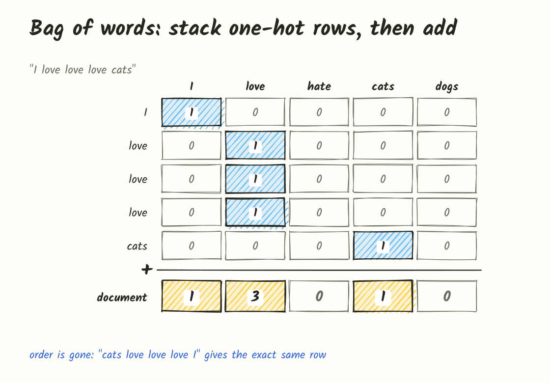
Vocabulary: ["I", "love", "hate", "cats", "dogs", "and"]

"I love cats and dogs"   → [1, 1, 0, 1, 1, 1]
"I hate cats"            → [1, 0, 1, 1, 0, 0]
"I love love love cats"  → [1, 3, 0, 1, 0, 0]

In scikit-learn this is CountVectorizer:

from sklearn.feature_extraction.text import CountVectorizer

docs = [
    "I love cats and dogs",
    "I hate cats",
    "I love love love cats",
]

vectorizer = CountVectorizer()
X = vectorizer.fit_transform(docs)

print(vectorizer.get_feature_names_out())
# ['and' 'cats' 'dogs' 'hate' 'love']

print(X.toarray())
# [[1 1 1 0 1]
#  [0 1 0 1 0]
#  [0 1 0 0 3]]

Notice that “I” isn’t in the vocabulary. The default tokenizer ignores tokens shorter than two characters. That’s usually fine, but if single characters matter in your data (sizes, grades, variable names), change token_pattern.

Everything is also lowercased and the columns are sorted alphabetically. The order of the columns doesn’t mean anything.

X is a sparse matrix. A real document uses a few hundred words out of tens of thousands, so storing only the non-zero values saves a lot of memory.

This is already useful. Documents that mention cats share a column, so their dot product is positive. A logistic regression on these counts makes a decent spam filter or topic classifier. But there are three problems.

Word order is gone. “Dog bites man” and “man bites dog” give exactly the same vector:

CountVectorizer().fit_transform(["dog bites man", "man bites dog"]).toarray()
# [[1 1 1]
#  [1 1 1]]

You can get some order back with ngram_range=(1, 2), which adds word pairs as extra columns. I wrote about that in the N-grams post.

There’s no notion of meaning. “Good” and “great” are separate columns. If the model learns that “great” is positive, it learns nothing about “good”.

Common words take over. Words like “the”, “is” and “a” show up in every document with high counts. They add to every vector while saying almost nothing about the topic. Stop-word lists help, but someone has to maintain them, and TF-IDF solves the same problem more cleanly.

TF-IDF

TF-IDF stands for term frequency, inverse document frequency. It keeps the bag of words layout but changes the numbers. Instead of a raw count, each word gets a weight that says how specific that word is to this document.

It multiplies two things.

Term frequency (TF) is how often the word appears in this document. That’s the bag of words count.

Inverse document frequency (IDF) is how rare the word is across all documents. If a word is in every document, it can’t help you tell documents apart, so its weight goes down. For $n$ documents, where the term $t$ appears in $\text{df}(t)$ of them:

A word in every document gets $\log 1 = 0$. A word in one document out of a thousand gets $\log 1000 \approx 6.9$.

Then:

So “the” might have a high count, but its IDF is close to zero and the product ends up small. A word like “delicious” only shows up in a few reviews, so when it does appear it gets a high score. It does the job of a stop-word list without needing a list.

scikit-learn uses a slightly different formula by default:

The $+1$ inside avoids dividing by zero. The $+1$ outside means a word that appears everywhere gets a weight of 1 instead of 0, so it’s pushed down but not removed. Each row is then L2-normalized so long and short documents can be compared.

Here’s what that looks like on three short reviews:

from sklearn.feature_extraction.text import TfidfVectorizer

docs = [
    "The food was delicious and amazing",
    "The service was terrible and slow",
    "The food was okay but expensive",
]

vectorizer = TfidfVectorizer()
X = vectorizer.fit_transform(docs)

The IDF values fall into three groups:

Word	Appears in	IDF
the, was	3 of 3 docs	1.00
and, food	2 of 3 docs	1.29
delicious, terrible, expensive, …	1 of 3 docs	1.69

And these are the weights for the first review:

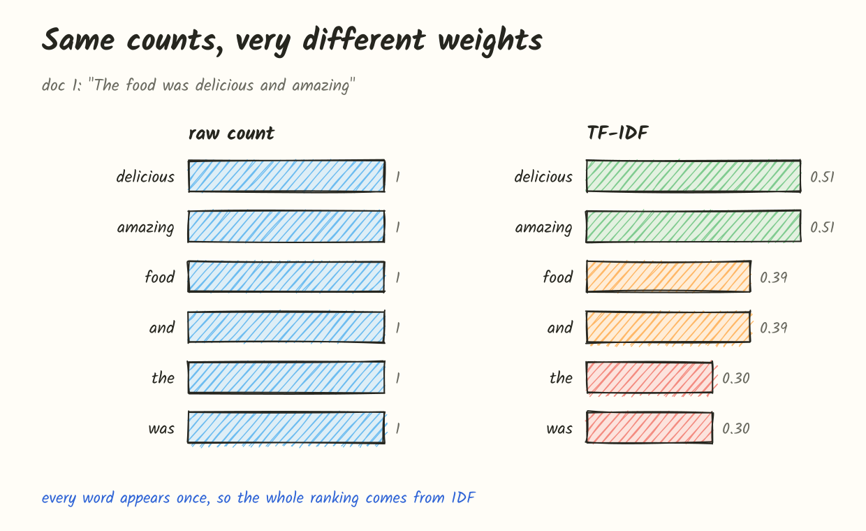
Every word appears once in that review, so the counts are all equal. The difference comes entirely from IDF. “Delicious” and “amazing” are the words that make this review different from the other two, and they end up on top.

With three documents the gap is small. With a million documents, “the” stays near 1 while a rare technical term can go above 10.

TF-IDF is still widely used. A close relative called BM25 adds two tweaks: repeated occurrences of a word count for less and less, and long documents don’t get an unfair advantage. BM25 is the default ranking in Elasticsearch, OpenSearch and Lucene, and it’s still hard to beat in a lot of search benchmarks.

It still doesn’t know about word order or meaning, though. “Good” and “great” remain unrelated columns.

HashingVectorizer

One more sparse method before moving on. This one solves a practical problem the others have.

CountVectorizer and TfidfVectorizer both work in two steps:

1. Go through the whole corpus and build a dictionary like {"the": 0, "cat": 1, "sat": 2, ...}.
2. Use that dictionary to turn each document into a vector.

The dictionary causes the trouble. A million documents can easily have 500,000 unique words, and the whole mapping has to fit in memory. You can’t start until you’ve seen all the data. You also have to save the vocabulary and ship it with the model. And a word that shows up for the first time at prediction time has no column, so it’s silently dropped.

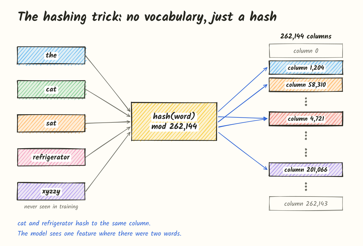
The hashing trick gets rid of the dictionary. Instead of looking up a word’s column, you calculate it:

$h$ is a hash function and $m$ is the number of columns you pick up front. scikit-learn uses 32-bit MurmurHash3, and n_features defaults to $2^{20}$, about a million columns. Any word, including one you’ve never seen, lands somewhere in that range.

from sklearn.feature_extraction.text import HashingVectorizer

vec = HashingVectorizer(n_features=2**18, alternate_sign=False, norm="l2")
X = vec.transform(docs)   # transform, not fit_transform: there's nothing to fit

You get the same kind of sparse matrix as CountVectorizer, but the column numbers don’t mean anything. On the cat example from earlier, “cats” goes to column 137,410 in all three rows and “love” goes to 148,489. Those numbers are arbitrary, but the same word always gets the same column, and that’s all the model needs.

Why you’d use it

• Nothing to fit or save. The vectorizer is just its parameters. You can recreate it anywhere.
• It works on streams. Vectorize one batch at a time and train with partial_fit, without loading the whole corpus.
• Memory doesn’t grow with vocabulary. A million documents or a billion, same memory.
• Easy to parallelize. Every worker computes the same columns without sharing any state.
• New words aren’t dropped. They get a column like everything else.

Here’s what streaming training looks like:

from sklearn.linear_model import SGDClassifier

vec = HashingVectorizer(n_features=2**20)
clf = SGDClassifier(loss="log_loss")

for texts, labels in batches():          # any iterator of mini-batches
    clf.partial_fit(vec.transform(texts), labels, classes=[0, 1])

What it costs

Collisions. Two different words can end up in the same column, and then the model can’t tell them apart.

This happens more than people expect. With 100,000 distinct words and $2^{20}$ columns, the chance that a given word shares its column with some other word is about:

That’s around 4,800 colliding pairs. In practice it matters less than it sounds. Most words are rare, so most collisions are between two rare words, or a common word and a rare one. The common word dominates the column and the rare one just adds a bit of noise. If you think collisions are hurting accuracy, increase n_features. Doubling it roughly halves the collision rate.

You can’t go back from a column to a word. Hashing is one-way, so you can’t inspect coefficients or see which words drove a prediction. For a lot of teams this is the real reason not to use it.

No IDF. Document frequency needs a count over the whole corpus, which is exactly the global state hashing avoids. You can add a TfidfTransformer after it, but that has to be fitted, so you lose most of the benefit.

alternate_sign. It’s True by default. A second hash decides whether each count is added or subtracted, so when two words collide their values partly cancel instead of stacking up. The downside is negative values. Set it to False if your model needs non-negative input, like multinomial Naive Bayes or NMF.

The name is a bit confusing. This isn’t hashing for hash tables or for cryptography. The hash function is only used to spread words across a fixed number of columns.

Which sparse vectorizer to pick

Situation	Use
Dataset fits in memory, you want interpretability	TfidfVectorizer
You need to know which words matter	TfidfVectorizer
Huge or streaming corpus	HashingVectorizer
Online learning with partial_fit	HashingVectorizer
Semantic similarity, paraphrases	Neither, use embeddings

That last row is the limit of everything so far. Hashing is still bag of words. “The food was not bad” and “the food was bad” share four of five words and get a cosine similarity close to 0.9. “Car” and “automobile” share nothing and get 0. These methods know which words appear, not what they mean.

Word embeddings

In every method so far, each word gets its own column. That’s why “good” and “great” can never be similar: they’re on different axes.

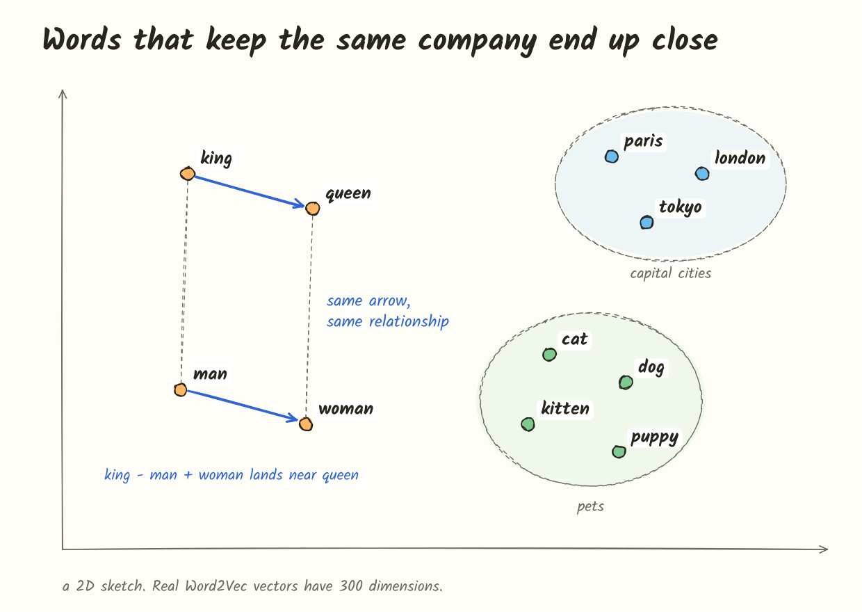
Word embeddings do it differently. Each word gets a short, dense vector, usually 100 to 300 numbers, and every word uses the same dimensions. The values aren’t assigned by hand. They’re learned, and they’re learned so that words used in similar contexts get similar vectors.

The idea is old. The linguist J. R. Firth put it as “you shall know a word by the company it keeps”. “Cat” and “dog” both appear near words like “pet”, “vet” and “fur”. “Paris” and “London” both appear near “capital”, “flight” and “mayor”. If you train a model to predict a word’s neighbors, words with similar neighbors end up with similar vectors.

How Word2Vec learns

Word2Vec came out of Google in 2013 (Mikolov et al.). Its skip-gram version slides a window over a large corpus, and for each word it tries to predict the words around it.

Every word $w$ has a vector $\mathbf{v}_w$. The model scores how likely a context word $c$ is using a dot product:

The bottom of that fraction sums over the whole vocabulary, which is far too slow to do for every training pair. Word2Vec uses negative sampling instead: push the score of the real neighbor up, and push the scores of a few random words down. Now each step is “which of these six words is the real neighbor?” instead of “which of 3 million words is it?”, and that’s cheap enough to run over billions of words.

The predictions themselves aren’t the goal. After training you throw away the prediction layer and keep the vectors.

GloVe, from Stanford in 2014, gets similar results another way. It first counts how often words appear near each other across the whole corpus, then fits vectors whose dot products match the log of those counts. The vectors you get behave about the same as Word2Vec’s.

What the vectors look like

These numbers are made up and cut down to a few dimensions, just to show the pattern:

"king"  → [ 0.91, 0.73, 0.55, -0.11, 0.62, ...]
"queen" → [ 0.89, 0.71, 0.53, -0.09, 0.60, ...]
"man"   → [ 0.45, 0.38, 0.21,  0.78, 0.11, ...]
"woman" → [ 0.43, 0.36, 0.19,  0.76, 0.09, ...]
"cat"   → [-0.22, 0.61, 0.87,  0.44, 0.33, ...]
"dog"   → [-0.20, 0.63, 0.85,  0.42, 0.35, ...]

Related words have similar vectors, so their cosine similarity is high. Don’t expect a single dimension to mean something like “royalty” or “animal”, though. The meaning is spread across all the dimensions. It shows up in distances and directions, not in individual numbers.

The king and queen example

Directions in the space also carry meaning. The direction from “man” to “woman” is roughly the same as the direction from “king” to “queen”. That’s why this works:

The same thing works for countries and capitals, verb tenses, and so on. You can try it with Google’s pre-trained vectors, which cover 3 million words and phrases with 300 dimensions each:

import gensim.downloader as api

model = api.load("word2vec-google-news-300")   # about 1.6 GB download

model["cat"].shape
# (300,)

model.most_similar("cat", topn=4)
# nearest neighbors: cats, dog, kitten, feline

model.most_similar(positive=["king", "woman"], negative=["man"], topn=1)
# [('queen', 0.7118...)]

One caveat: most_similar never returns the words you passed in. Without that filter, the closest vector to king - man + woman is often “king” itself, since adding and subtracting two similar vectors doesn’t move you far. The relationship is real, but the demo makes it look a bit cleaner than it is.

Embeddings also pick up biases from their training text. The same arithmetic that finds “queen” will just as happily reproduce gender stereotypes about jobs.

Where word embeddings fall short

One vector per word. “Bank” in “river bank” and in “bank account” gets the same vector, a mix of both meanings.

Unknown words have no vector. Typos, new product names and rare word forms just aren’t there. fastText (Facebook, 2016) helps by building word vectors from pieces of words, so it can put together a vector for “unfriendliness” from parts it has seen.

They don’t give you sentence vectors. The obvious fix is to average the word vectors in a sentence. That’s a reasonable baseline, but it loses word order just like bag of words did. “Dog bites man” and “man bites dog” average to the same thing.

Sentence embeddings

Transformer models like BERT (2018) changed this. A transformer doesn’t look up a fixed vector per word. It computes each token’s vector from the whole sentence using attention. “Bank” next to “river” and “bank” next to “loan” get different vectors. These are called contextual embeddings.

That still gives one vector per token. For search, clustering, deduplication or RAG, you usually want one vector for the whole sentence or paragraph.

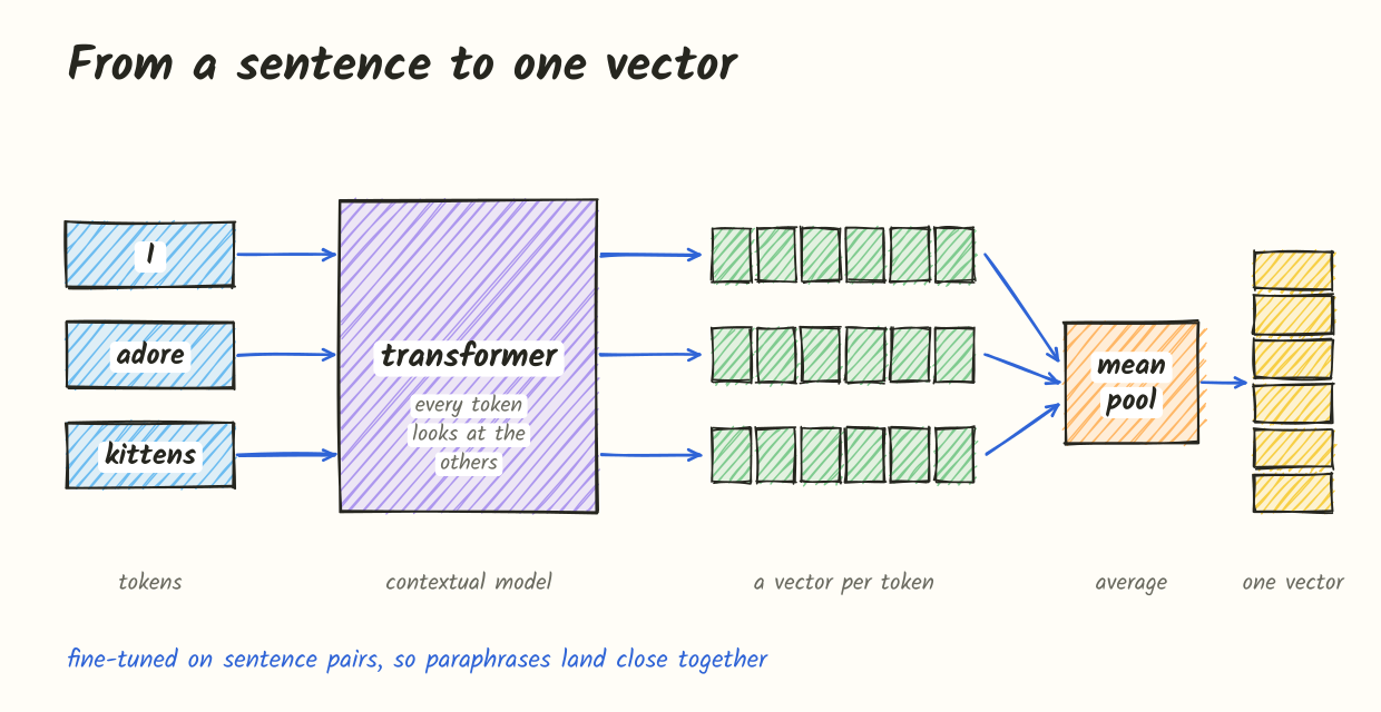
Averaging BERT’s token vectors doesn’t work very well on its own. BERT was trained to fill in masked words. Nothing in that training makes similar sentences land close together.

Sentence-BERT (Reimers and Gurevych, 2019) fixed that by fine-tuning on pairs of sentences. Pairs with the same meaning get pulled together and unrelated sentences get pushed apart. The token vectors are then averaged into one fixed-size vector. After this training, cosine similarity between two sentence vectors actually tracks how similar their meanings are.

The sentence-transformers library handles all of it:

from sentence_transformers import SentenceTransformer

model = SentenceTransformer("all-MiniLM-L6-v2")

sentences = [
    "I love cats",
    "I adore kittens",
    "The stock market fell",
]

embeddings = model.encode(sentences, normalize_embeddings=True)
embeddings.shape
# (3, 384)

similarity = model.similarity(embeddings, embeddings)
# "I love cats" vs "I adore kittens"       → high
# "I love cats" vs "The stock market fell" → close to zero

“I love cats” and “I adore kittens” don’t share a single content word. Every sparse method in this post would say they’re unrelated. The embedding model puts them close together because it has learned that “love” and “adore” are used the same way, and that kittens are cats.

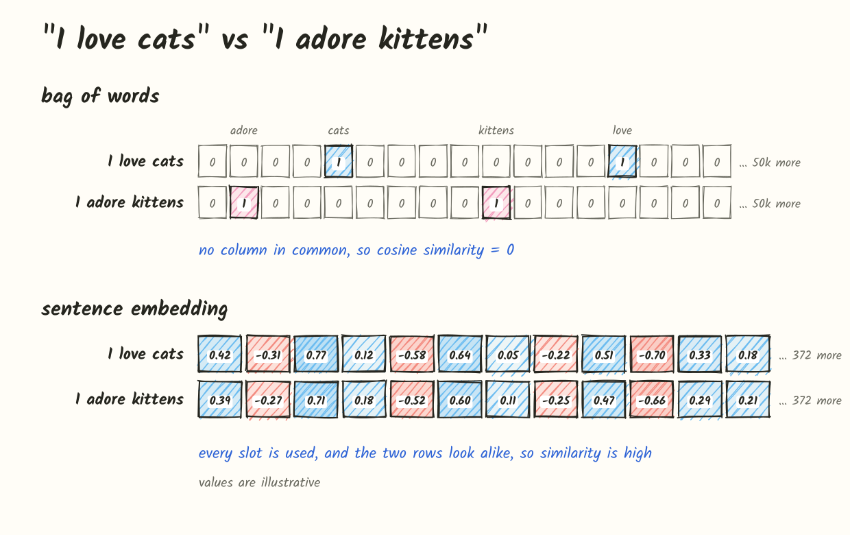
all-MiniLM-L6-v2 gives 384-dimensional vectors and runs fine on a CPU, which is why it’s in so many tutorials. Bigger open models like all-mpnet-base-v2 give 768 dimensions and do noticeably better. Hosted APIs go further: OpenAI’s text-embedding-3-small returns 1,536 dimensions and text-embedding-3-large returns 3,072. Many newer models are trained so you can keep only the first few hundred dimensions without losing much accuracy, which saves storage.

A few things that will save you debugging time:

• Normalize your vectors and use the dot product. For unit-length vectors, the dot product is the same as cosine similarity and faster. Most vector databases expect this.
• Don’t mix vectors from different models. Two models produce unrelated spaces, even with the same number of dimensions. If you switch models, re-embed everything.
• Watch the input length. Models have a maximum length and cut off anything past it without warning. all-MiniLM-L6-v2 stops at 256 tokens, so long documents need to be split into chunks first.
• Check whether the model wants prefixes. Some models, like the E5 family, expect "query: " and "passage: " in front of the text. Leave them out and retrieval gets noticeably worse. The model card will say.

All methods compared

Method	Vector type	Typical size	Captures meaning?	Interpretable?	Typical use
One-hot	Sparse, binary	Vocabulary size	No	Yes	Input to embedding layers
Bag of words	Sparse, counts	Vocabulary size	No	Yes	Simple classification baselines
TF-IDF / BM25	Sparse, weighted	Vocabulary size	No	Yes	Keyword search, classification
Hashing	Sparse, hashed	Fixed, ~$2^{18}$ to $2^{20}$	No	No	Streaming, huge corpora
Word2Vec / GloVe	Dense	100 to 300	Per word, no context	No	Word similarity, older pipelines
Sentence embeddings	Dense	384 to 3,072	Yes, in context	No	Semantic search, clustering, RAG

Lower rows understand meaning better. They also cost more to compute, are harder to inspect, and are worse at matching exact strings.

Using sparse and dense together

You might expect embeddings to have replaced the older methods. They haven’t, because sparse and dense vectors fail in opposite ways.

Embeddings handle paraphrases well but struggle with exact identifiers. Search for the error code E_CONN_4012, the SKU XR-7719-B or an unusual surname, and semantic search might return pages about connection errors or products in general, ranked above the one page that contains that exact string.

Sparse matching is the opposite. It will never connect “car” with “automobile”, but it always finds the exact token you typed.

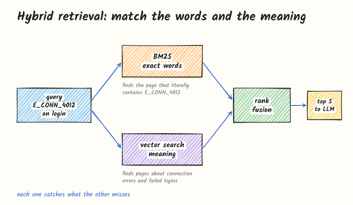
That’s why the older methods still show up in AI systems:

• Hybrid retrieval. Run BM25 and vector search side by side, then merge the two rankings, often with reciprocal rank fusion. This is now the standard advice for RAG, because you catch both paraphrases and exact identifiers.
• Cheap filters before an LLM call. A linear classifier on hashed or TF-IDF features can flag spam or abuse in microseconds on a CPU. Put it in front of your LLM and you don’t pay to process obvious junk.
• Near-duplicate detection. Split documents into overlapping N-grams and compare them with MinHash or SimHash. It scales to billions of documents and is the usual way to deduplicate training and fine-tuning data.
• Cost. Hashing and TF-IDF are basically free. Embedding a hundred million passages costs real money and GPU time, and you pay again every time you change models. Check whether the cheap option is good enough before paying for the expensive one.

Picking one

All of these methods answer the same question: when should two pieces of text count as similar?

• One-hot: never.
• Bag of words: when they use the same words.
• TF-IDF: when they share the same uncommon words.
• Word embeddings: when their words appear in similar contexts.
• Sentence embeddings: when they mean the same thing.

Each step down that list understands language better, and each one costs more and is harder to inspect. So the newest method isn’t automatically the right one. Searching product codes needs exact matches. A support bot that has to connect “my card got declined” with “payment failure troubleshooting” needs meaning. Most real systems need both.